Lokale Darstellbarkeit durch Graphen
Question
Solution
Short
Video
\(\LaTeX\)

No explanation / solution video to this exercise has yet been created.
Visit our YouTube-Channel to see solutions to other exercises.
Don't forget to subscribe to our channel, like the videos and leave comments!
Visit our YouTube-Channel to see solutions to other exercises.
Don't forget to subscribe to our channel, like the videos and leave comments!
Exercise:
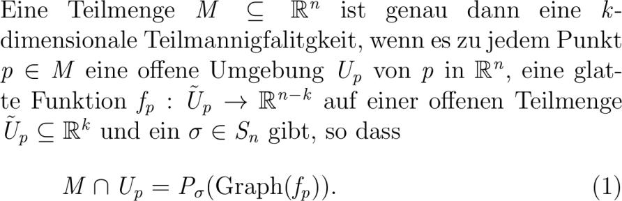
Eine Teilmenge Msubseteq mathbbR^n ist genau dann eine k-dimensionale Teilmannigfalitgkeit wenn es zu jedem Punkt pin M eine offene Umgebung U_p von p in mathbbR^n eine glatte Funktion f_p:tildeU_prightarrow mathbbR^n-k auf einer offenen Teilmenge tildeU_p subseteq mathbbR^k und ein sigmain S_n gibt so dass Mcap U_p P_sigmatextGraphf_p.
Solution:
Beweis. Angenommen M ist eine k-dimensionale Teilmannigfaltigkeit. Sei pin M U_p eine offene Umgebung von pin mathbbR^n und phi_p: U_prightarrow V_psubseteq mathbbR^n ein Diffeomorphismus wie in Definition . mit phi_pp. Sei psi:y_...y_kin -epsilon epsilon^kmapsto phi_p^-y_...y_k...in M für ein epsilon klein genug. Dann hat das Differential textD_phi Rang k womit k linear unabhängige Zeilen in textD_psi existieren. Nach Koordinatenvertauschung von hier stammt sigma in der Aussage kann man annehmen dass diese Zeilen die ersten k sind. Damit hat die Abbildung g:yin -epsilon epsilon^kmapsto psi_y...psi_ky^t ein invertierbares Differential bei . Also existiert nach dem Satz zur inversen Abbildung Satz . eine nicht-leere offene Menge Usubseteq -epsilon epsilon^k so dass die Einschränkung von g auf U ein Diffeomorphismus ist. Man betrachtet nun die Abbildung fpsicirc g|_U^-:gUrightarrow M. Für ileq k und alle yin gU gilt f_iypsi_ig|_U^-yy_i nach Konstruktion. Die Teilmannigfaltigkeit M ist also lokal der Graph der Abbildung yin gUmapsto f_k+y...f_ny nach Permutation der Koordinaten womit der erste Teil der Aussage bewiesen ist. Für die Umkehrung kann man analog vorgehen wie in Beispiel .c.