TeXercises.com

Non-Stationary State

About points...

We associate a certain number of points with each exercise.
When you click an exercise into a collection, this number will be taken as points for the exercise, kind of "by default".
But once the exercise is on the collection, you can edit the number of points for the exercise in the collection independently, without any effect on "points by default" as represented by the number here.

That being said... How many "default points" should you associate with an exercise upon creation?
As with difficulty, there is no straight forward and generally accepted way.
But as a guideline, we tend to give as many points by default as there are mathematical steps to do in the exercise.
Again, very vague... But the number should kind of represent the "work" required.

About difficulty...

We associate a certain difficulty with each exercise.
When you click an exercise into a collection, this number will be taken as difficulty for the exercise, kind of "by default".
But once the exercise is on the collection, you can edit its difficulty in the collection independently, without any effect on the "difficulty by default" here.
Why we use chess pieces? Well... we like chess, we like playing around with \(\LaTeX\)-fonts, we wanted symbols that need less space than six stars in a table-column... But in your layouts, you are of course free to indicate the difficulty of the exercise the way you want.

That being said... How "difficult" is an exercise? It depends on many factors, like what was being taught etc.
In physics exercises, we try to follow this pattern:

Level 1 - One formula (one you would find in a reference book) is enough to solve the exercise. Example exercise

Level 2 - Two formulas are needed, it's possible to compute an "in-between" solution, i.e. no algebraic equation needed. Example exercise

Level 3 - "Chain-computations" like on level 2, but 3+ calculations. Still, no equations, i.e. you are not forced to solve it in an algebraic manner. Example exercise

Level 4 - Exercise needs to be solved by algebraic equations, not possible to calculate numerical "in-between" results. Example exercise

Level 5 -
Level 6 -

Exercise

https://texercises.com/exercise/non-stationary-state/

Question

Solution

Short

Video

\(\LaTeX\)

No explanation / solution video to this exercise has yet been created.

Visit our YouTube-Channel to see solutions to other exercises.
Don't forget to subscribe to our channel, like the videos and leave comments!

Exercise:
Derive the probability density for the state psixt fracsqrtpsi_xt+fracsqrtpsi_xt of the infinite potential well. Compare the result to the probability density of a stationary state.

Solution:
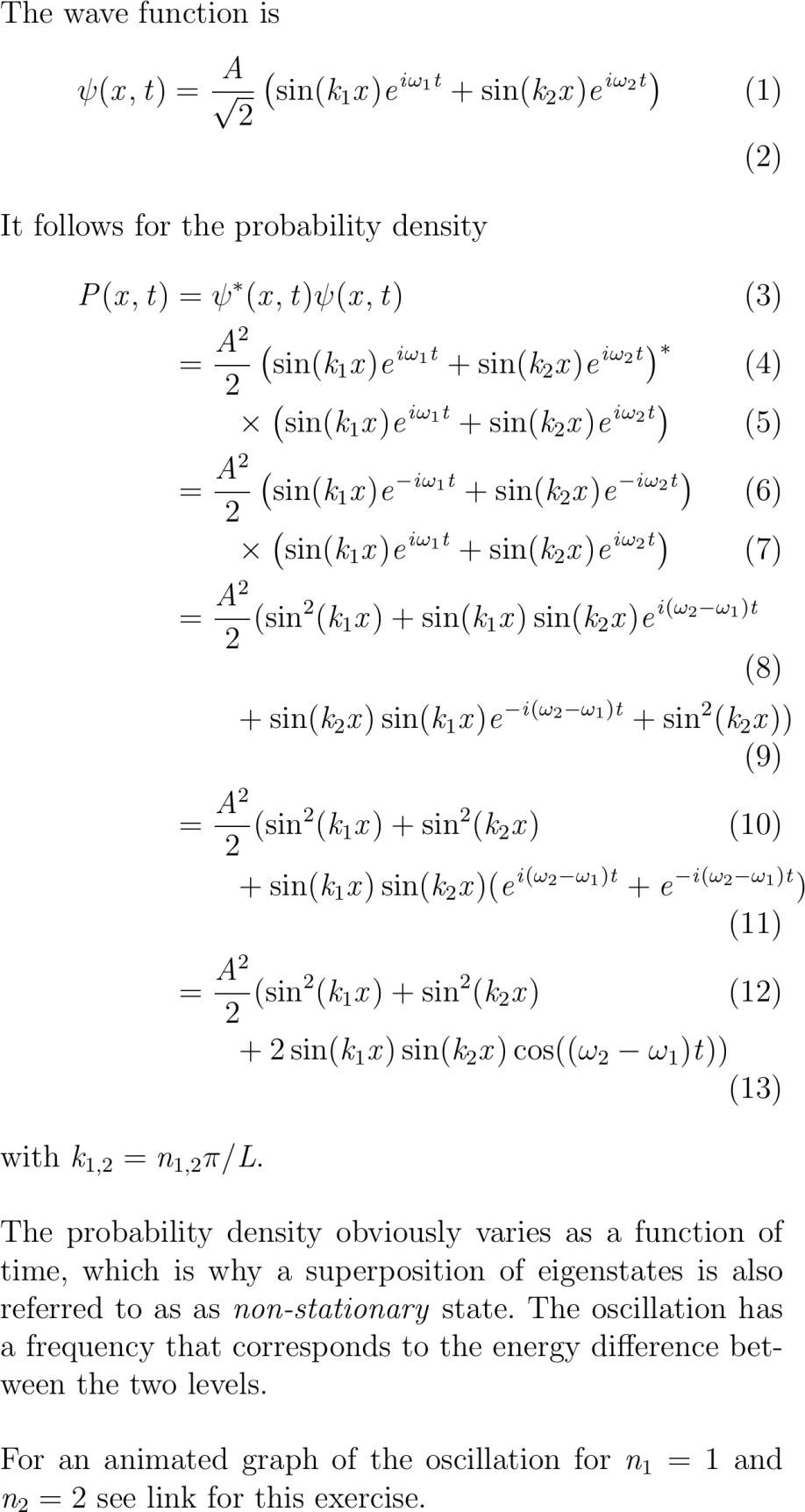
The wave function is psixt fracAsqrtleftsink_ xe^iomega_ t+sink_ xe^iomega_ t right It follows for the probability density Pxt psi^*xtpsixt fracA^leftsink_ xe^iomega_ t+sink_ xe^iomega_ t right^* &qquad timesleftsink_ xe^iomega_ t+sink_ xe^iomega_ t right fracA^leftsink_ xe^-iomega_ t+sink_ xe^-iomega_ t right &qquad times leftsink_ xe^iomega_ t+sink_ xe^iomega_ t right fracA^ sin^k_ x+sink_ xsink_ x e^iomega_-omega_t &qquad + sink_ xsink_ x e^-iomega_-omega_t + sin^k_ x fracA^sin^k_ x+sin^k_ x &qquad + sink_ xsink_ xe^iomega_-omega_t+e^-iomega_-omega_t fracA^sin^k_ x+sin^k_ x &qquad + sink_ xsink_ xcosomega_-omega_t with k_n_pi/L. vspacemm The probability density obviously varies as a function of time which is why a superposition of eigenstates is also referred to as as non-stationary state. The oscillation has a frequency that corresponds to the energy difference between the two levels. vspacemm For an animated graph of the oscillation for n_ and n_ see link for this exercise.

Meta Information

\(\LaTeX\)-Code

Contained in these collections:

Schrödinger Equation by by

4 | 10

Attributes & Decorations

Branches	quantum physics
Tags	energy level, probability density
Content image
Difficulty	(2, default)
Points	0 (default)
Language	(English)
Type	Calculative / Quantity
Creator	by
Decoration
File
Link	Probability Density 1 – 2