Reduzierter Kreisprozess
Question
Solution
Short
Video
\(\LaTeX\)

No explanation / solution video to this exercise has yet been created.
Visit our YouTube-Channel to see solutions to other exercises.
Don't forget to subscribe to our channel, like the videos and leave comments!
Visit our YouTube-Channel to see solutions to other exercises.
Don't forget to subscribe to our channel, like the videos and leave comments!
Exercise:
In einem Zylinder mit verschiebbarem Kolben befinden sich .mol eines zweiatomigen Gases der Temperatur T_A K und dem augenblicklichen Volumen V_A .decim^. Zuerst wird das Gas adiabatisch auf das Volumen V_B .decim^ expandiert; danach wird es isotherm auf den Anfangsdruck p_A komprimiert um schliesslich durch eine isobare Expansion in den Anfangszustand zurückgeführt zu werden. enumerate item Skizzieren Sie diesen Kreisprozess in einem pV-Diagramm und schreiben Sie die gegebenen Grössen an. ~Pkte item Berechnen Sie die fehlen Druck- p_Ap_Bp_C Volumen- V_C bzw. Temperaturwerte T_B T_C für diesen Kreisprozess. ~Pkte item Berechnen Sie die zugeführte bzw. weggeführte Wärmemenge. ~Pkt item Berechnen Sie die pro Umlauf verrichtete Arbeit. ~Pkte item Bestimmen Sie den Wirkungsgrad dieser Wärmekraftmaschine und vergleichen Sie ihn mit dem Carnot-Wirkungsgrad. ~Pkte enumerate
Solution:
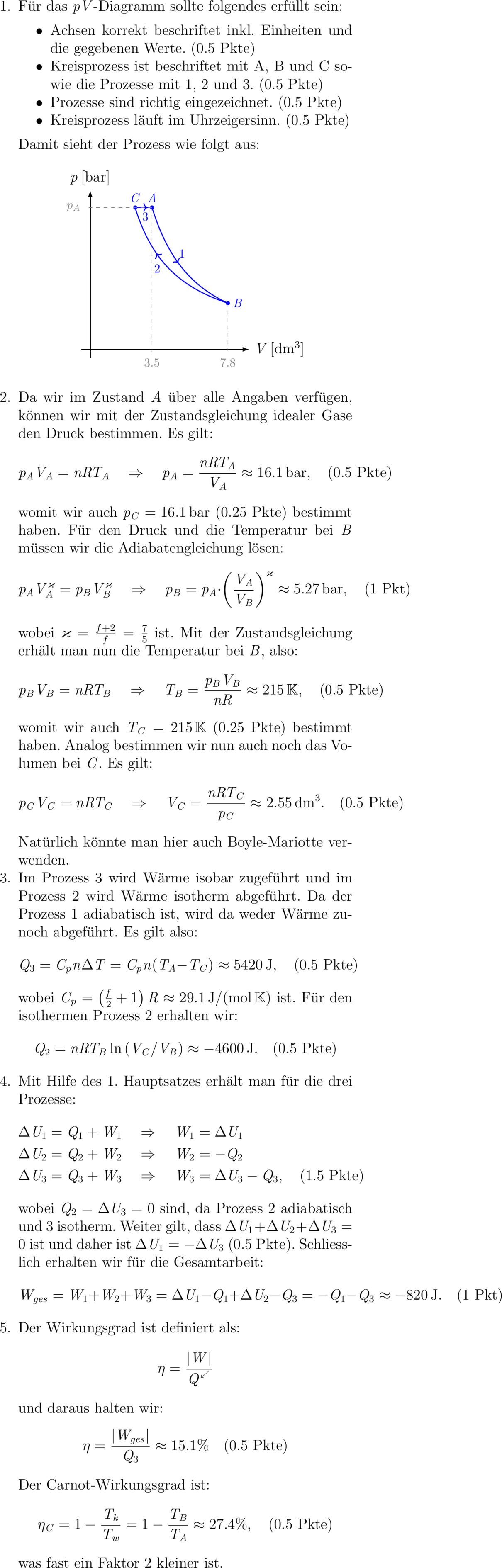
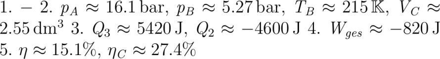
enumerate item Für das pV-Diagramm sollte folges erfüllt sein: itemize item Achsen korrekt beschriftet inkl. Einheiten und die gegebenen Werte. .~Pkte item Kreisprozess ist beschriftet mit A B und C sowie die Prozesse mit und . .~Pkte item Prozesse sind richtig eingezeichnet. .~Pkte item Kreisprozess läuft im Uhrzeigersinn. .~Pkte itemize Damit sieht der Prozess wie folgt aus: center tikzpicturescale. % Koordinatensystem draw thick-latex -. -- node right Vdecim^; draw thick-latex -. -- node above pbbar; % Prozess Punkte draw fillblueblue .. node above fns A circle mm; draw fillblueblue .. node right fns B circle mm; draw fillblueblue .. node above fns C circle mm; % Prozess adiabate draw domain.:.thick blue plotidadia samples x./x^/; draw domain.:thick blu plotidadia samples x./x^/ node abovexshiftmmfns ; % Prozess isotherme draw domain.:.thick blue plotidadia samples x./x; draw domain.:thick blue- plotidadia samples x./x node belowxshift-mmfns ; % Prozess isobar draw thickblu . -- node below fns ++ .; draw thickblue .. -- ..; % Hilfslinien draw dashedgray .. -- .-. node below fns .; draw dashedgray .. -- .-. node below fns .; draw dashedgray .. -- -.. node left fns p_A; tikzpicture center item Da wir im Zustand A über alle Angaben verfügen können wir mit der Zustandsgleichung idealer Gase den Druck bestimmen. Es gilt: p_AV_A nRT_A myRarrow p_A fracnRT_AV_A apx .bbar quad text.~Pkte womit wir auch p_C .bbar .~Pkte bestimmt haben. Für den Druck und die Temperatur bei B müssen wir die Adiabatengleichung lösen: p_AV_A^kappa p_BV_B^kappa myRarrow p_B p_A leftfracV_AV_Bright^kappa apx .bbar quad text~Pkt wobei kappa fracf+f frac ist. Mit der Zustandsgleichung erhält man nun die Temperatur bei B also: p_BV_B nRT_B myRarrow T_B fracp_BV_BnR apx K quad text.~Pkte womit wir auch T_C K .~Pkte bestimmt haben. Analog bestimmen wir nun auch noch das Volumen bei C. Es gilt: p_CV_C nRT_C myRarrow V_C fracnRT_Cp_C apx .decim^. quad text.~Pkte Natürlich könnte man hier auch BoylMariotte verwen. item Im Prozess wird Wärme isobar zugeführt und im Prozess wird Wärme isotherm abgeführt. Da der Prozess adiabatisch ist wird da weder Wärme zu- noch abgeführt. Es gilt also: Q_ C_p n Delta T C_p n T_A - T_C apx J quad text.~Pkte wobei C_p leftfracf+rightR apx .J/molK ist. Für den isothermen Prozess erhalten wir: Q_ nRT_B ln leftV_C/V_Bright apx -J. quad text.~Pkte item Mit Hilfe des . Hauptsatzes erhält man für die drei Prozesse: eqnarray* Delta U_ & Q_ + W_ myRarrow W_ Delta U_ Delta U_ & Q_ + W_ myRarrow W_ - Q_ Delta U_ & Q_ + W_ myRarrow W_ Delta U_ - Q_ quad text.~Pkte eqnarray* wobei Q_ Delta U_ sind da Prozess adiabatisch und isotherm. Weiter gilt dass Delta U_ + Delta U_ + Delta U_ ist und daher ist Delta U_ -Delta U_ .~Pkte. Schliesslich erhalten wir für die Gesamtarbeit: W_ges W_ + W_ + W_ Delta U_ - Q_ + Delta U_ - Q_ -Q_ - Q_ apx -J.quad text~Pkt item Der Wirkungsgrad ist definiert als: eta frac|W|Q^^swarrow und daraus halten wir: eta frac|W_ges|Q_ apx .%quad text.~Pkte Der Carnot-Wirkungsgrad ist: eta_C -fracT_kT_w - fracT_BT_A apx .%quad text.~Pkte was fast ein Faktor kleiner ist. enumerate
In einem Zylinder mit verschiebbarem Kolben befinden sich .mol eines zweiatomigen Gases der Temperatur T_A K und dem augenblicklichen Volumen V_A .decim^. Zuerst wird das Gas adiabatisch auf das Volumen V_B .decim^ expandiert; danach wird es isotherm auf den Anfangsdruck p_A komprimiert um schliesslich durch eine isobare Expansion in den Anfangszustand zurückgeführt zu werden. enumerate item Skizzieren Sie diesen Kreisprozess in einem pV-Diagramm und schreiben Sie die gegebenen Grössen an. ~Pkte item Berechnen Sie die fehlen Druck- p_Ap_Bp_C Volumen- V_C bzw. Temperaturwerte T_B T_C für diesen Kreisprozess. ~Pkte item Berechnen Sie die zugeführte bzw. weggeführte Wärmemenge. ~Pkt item Berechnen Sie die pro Umlauf verrichtete Arbeit. ~Pkte item Bestimmen Sie den Wirkungsgrad dieser Wärmekraftmaschine und vergleichen Sie ihn mit dem Carnot-Wirkungsgrad. ~Pkte enumerate
Solution:
enumerate item Für das pV-Diagramm sollte folges erfüllt sein: itemize item Achsen korrekt beschriftet inkl. Einheiten und die gegebenen Werte. .~Pkte item Kreisprozess ist beschriftet mit A B und C sowie die Prozesse mit und . .~Pkte item Prozesse sind richtig eingezeichnet. .~Pkte item Kreisprozess läuft im Uhrzeigersinn. .~Pkte itemize Damit sieht der Prozess wie folgt aus: center tikzpicturescale. % Koordinatensystem draw thick-latex -. -- node right Vdecim^; draw thick-latex -. -- node above pbbar; % Prozess Punkte draw fillblueblue .. node above fns A circle mm; draw fillblueblue .. node right fns B circle mm; draw fillblueblue .. node above fns C circle mm; % Prozess adiabate draw domain.:.thick blue plotidadia samples x./x^/; draw domain.:thick blu plotidadia samples x./x^/ node abovexshiftmmfns ; % Prozess isotherme draw domain.:.thick blue plotidadia samples x./x; draw domain.:thick blue- plotidadia samples x./x node belowxshift-mmfns ; % Prozess isobar draw thickblu . -- node below fns ++ .; draw thickblue .. -- ..; % Hilfslinien draw dashedgray .. -- .-. node below fns .; draw dashedgray .. -- .-. node below fns .; draw dashedgray .. -- -.. node left fns p_A; tikzpicture center item Da wir im Zustand A über alle Angaben verfügen können wir mit der Zustandsgleichung idealer Gase den Druck bestimmen. Es gilt: p_AV_A nRT_A myRarrow p_A fracnRT_AV_A apx .bbar quad text.~Pkte womit wir auch p_C .bbar .~Pkte bestimmt haben. Für den Druck und die Temperatur bei B müssen wir die Adiabatengleichung lösen: p_AV_A^kappa p_BV_B^kappa myRarrow p_B p_A leftfracV_AV_Bright^kappa apx .bbar quad text~Pkt wobei kappa fracf+f frac ist. Mit der Zustandsgleichung erhält man nun die Temperatur bei B also: p_BV_B nRT_B myRarrow T_B fracp_BV_BnR apx K quad text.~Pkte womit wir auch T_C K .~Pkte bestimmt haben. Analog bestimmen wir nun auch noch das Volumen bei C. Es gilt: p_CV_C nRT_C myRarrow V_C fracnRT_Cp_C apx .decim^. quad text.~Pkte Natürlich könnte man hier auch BoylMariotte verwen. item Im Prozess wird Wärme isobar zugeführt und im Prozess wird Wärme isotherm abgeführt. Da der Prozess adiabatisch ist wird da weder Wärme zu- noch abgeführt. Es gilt also: Q_ C_p n Delta T C_p n T_A - T_C apx J quad text.~Pkte wobei C_p leftfracf+rightR apx .J/molK ist. Für den isothermen Prozess erhalten wir: Q_ nRT_B ln leftV_C/V_Bright apx -J. quad text.~Pkte item Mit Hilfe des . Hauptsatzes erhält man für die drei Prozesse: eqnarray* Delta U_ & Q_ + W_ myRarrow W_ Delta U_ Delta U_ & Q_ + W_ myRarrow W_ - Q_ Delta U_ & Q_ + W_ myRarrow W_ Delta U_ - Q_ quad text.~Pkte eqnarray* wobei Q_ Delta U_ sind da Prozess adiabatisch und isotherm. Weiter gilt dass Delta U_ + Delta U_ + Delta U_ ist und daher ist Delta U_ -Delta U_ .~Pkte. Schliesslich erhalten wir für die Gesamtarbeit: W_ges W_ + W_ + W_ Delta U_ - Q_ + Delta U_ - Q_ -Q_ - Q_ apx -J.quad text~Pkt item Der Wirkungsgrad ist definiert als: eta frac|W|Q^^swarrow und daraus halten wir: eta frac|W_ges|Q_ apx .%quad text.~Pkte Der Carnot-Wirkungsgrad ist: eta_C -fracT_kT_w - fracT_BT_A apx .%quad text.~Pkte was fast ein Faktor kleiner ist. enumerate